library(gprofiler2)gProfiler (MOV10)
gProfileR es otra herramienta para realizar análisis de sobrerepresentación (ORA), similar a clusterProfiler. gProfileR considera multiples fuentes, incluidos los términos GO. Los términos GO resultantes son en general similares a los conseguidos con clusterProfiler, pero pude haber diferecias debido a los algoritmos usados.
Usando gProfileR
Cargamos los datos correspondientes a los genes DGE, y los ordenamos por FC
df.fc <- read.csv('../rnaseq/deseq/data/resultado.csv')
df.fc <- df.fc[order(df.fc$log2FoldChange, decreasing = TRUE), ]

padj.cutoff <- 0.05
lfc.cutoff <- log2(1.5)

genes.up <- df.fc$X[df.fc$log2FoldChange >= lfc.cutoff & df.fc$padj <= padj.cutoff]
genes.down <- df.fc$X[df.fc$log2FoldChange <= -1 * lfc.cutoff & df.fc$padj <= padj.cutoff]

genes.dge <- c(genes.up, genes.down)
allgenes <- df.fc$X
gost.res <- gost(query = genes.dge,
organism = 'hsapiens',
ordered_query = TRUE,
correction_method = 'fdr',
custom_bg = allgenes,
highlight = TRUE
)
head(gost.res$result, 3)| query | significant | p_value | term_size | query_size | intersection_size | precision | recall | term_id | source | term_name | effective_domain_size | source_order | parents |
|---|---|---|---|---|---|---|---|---|---|---|---|---|---|
| query_1 | TRUE | 0.0012102 | 2 | 35 | 2 | 0.0571429 | 1.0 | CORUM:6522 | CORUM | Harmonin-CAD23 complex | 13705 | 2197 | CORUM:0000000 |
| query_1 | TRUE | 0.0290175 | 2 | 405 | 2 | 0.0049383 | 1.0 | CORUM:1634 | CORUM | CyclinD1-CDK4-p21 complex | 13705 | 798 | CORUM:0000000 |
| query_1 | TRUE | 0.0290175 | 5 | 5 | 1 | 0.2000000 | 0.2 | CORUM:1874 | CORUM | SNARE complex (SNAP25, VAMP3, VAMP2, NAPB, STX13) | 13705 | 851 | CORUM:0000000 |
Visualizando resultados
gostplot(gost.res, capped = TRUE, interactive = TRUE)#| label: link
gost.link <- gost(query = genes.dge,
organism = 'hsapiens',
ordered_query = TRUE,
correction_method = 'fdr',
custom_bg = allgenes,
highlight = TRUE,
as_short_link = TRUE
)
gost.linkREVIGO
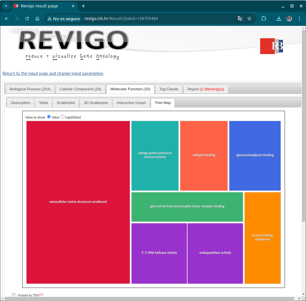
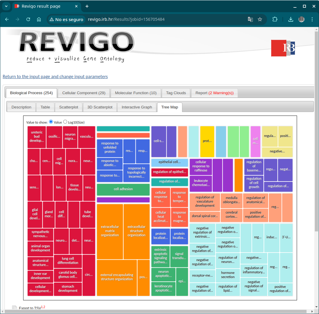
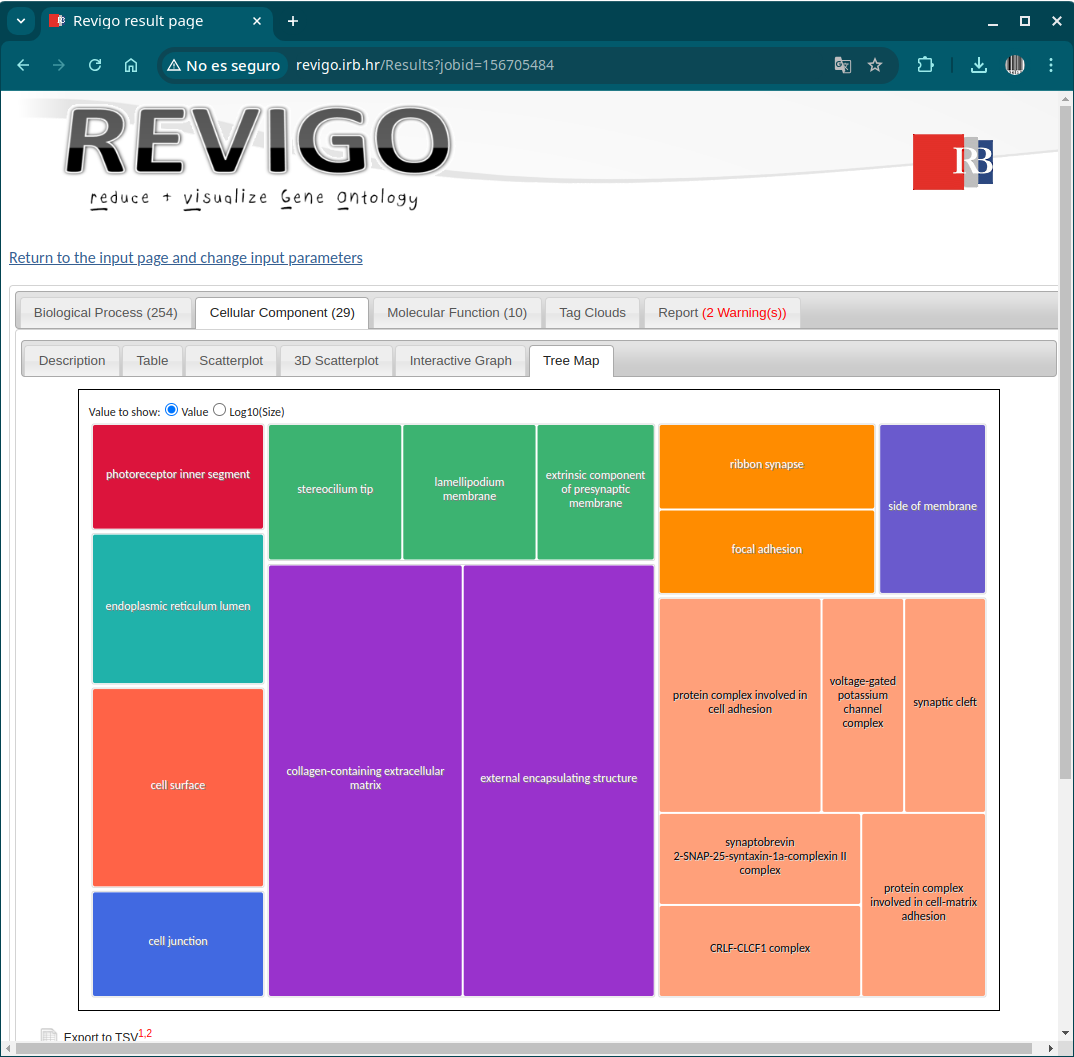
REVIGO es una herramienta web que resume graficamente la lista de términos GO déspues de eliminar los terminos redundantes.
gprofiler_results <- gost.res$result[order(gost.res$result$p_value, decreasing = TRUE),]
gprofiler_results <- gprofiler_results[grep('GO:', gprofiler_results$term_id), ]

GO.pval <- gprofiler_results[, c('term_id', 'p_value')]

write.table(GO.pval, "GOs_oe.txt", quote=FALSE, row.names = FALSE, col.names = FALSE)

head(GO.pval)| term_id | p_value | |
|---|---|---|
| 304 | GO:0098888 | 0.0496310 |
| 266 | GO:0021892 | 0.0493426 |
| 267 | GO:0150011 | 0.0493426 |
| 268 | GO:0099525 | 0.0493426 |
| 269 | GO:0090090 | 0.0493426 |
| 270 | GO:0001666 | 0.0493426 |
Abrimos el fichero ‘GOs_oe.txt’ y copiamos y pegamos su contenido en la web de REVIGO.
Procesos biológicos
Componentes celulares
Funciones moleculares